Sales Forecasting (Time-Series)

Overview

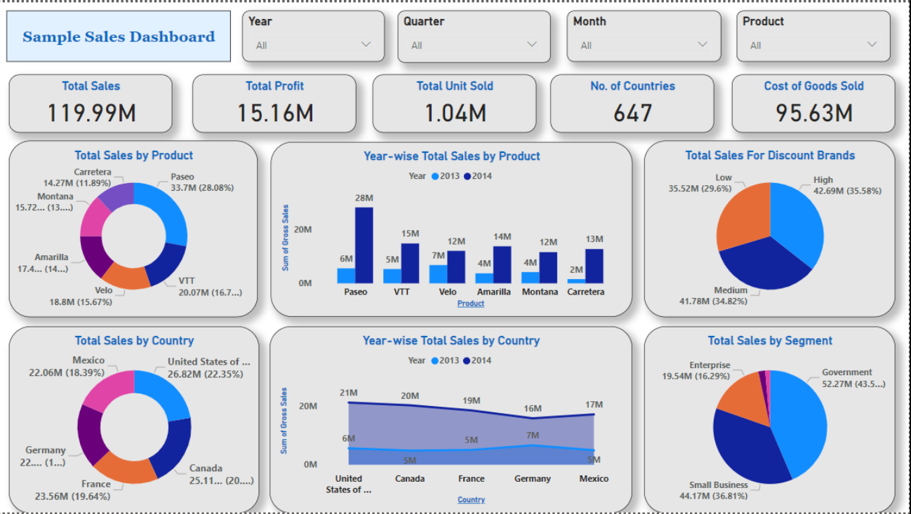
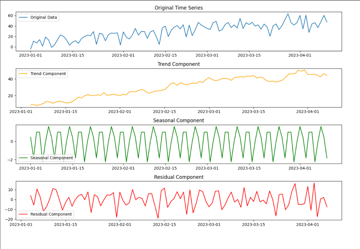
We built a forecasting pipeline that learns seasonality, promotions, holidays, and price elasticity to predict weekly sales per product–location. A Power BI dashboard visualizes forecasts, uncertainty, and bias, helping planners align inventory and campaigns.

Data

• Grain: weekly product × store (3–5 years history)
• Signals: calendar, holidays, promos, prices, weather, stockouts
• Targets: units and/or revenue; forecast horizon typically 8–12 weeks

Approach

• Baselines: Naïve, seasonal naïve, ETS.
• Classical: SARIMA / Prophet for strong weekly/annual seasonality.
• ML: Gradient boosting (XGBoost) with lags, rolling means, promo/price features.
• Validation: Rolling-origin time-series CV; metrics: MAPE/WAPE/sMAPE/RMSE.
• Ensemble: Blend classical + ML per series based on validation rank.

# sketch: lag/window features for ML
def add_lag_feats(df, lags=(1,2,3,4,5,6,7,14,28), windows=(7,28)):
    for L in lags:
        df[f"y_lag_{L}"] = df.groupby(["store","sku"])["y"].shift(L)
    for W in windows:
        df[f"y_ma_{W}"]  = (df.groupby(["store","sku"])["y"]
                             .shift(1).rolling(W, min_periods=1).mean())
    return df

# sketch: rolling-origin cross-validation
def rolling_cv(df, n_folds=4, horizon=8):
    folds = []
    end = df["ds"].max()
    for k in range(n_folds):
        cutoff = end - pd.Timedelta(weeks=(n_folds-k)*horizon)
        tr = df[df["ds"] <= cutoff]
        va = df[(df["ds"] > cutoff) & (df["ds"] <= cutoff + pd.Timedelta(weeks=horizon))]
        folds.append((tr, va))
    return folds

Tech Stack

Python · Pandas · Prophet / SARIMA · XGBoost · scikit-learn · Power BI · (optional) Power Automate